Paper Summary — RepVGG : Making VGG-style ConvNets Great Again
In this paper, the authors introduce RepVGG, a modified version of the VGG architecture with different Training/Inference architecture achieved via Reparameterisation. The authors show that how by using just stacking Convolution operations and ReLUs without branches(like in ResNet) or any other complex convolution operation(such as Group-wise covolution) can perform at par with models with complex architectures.
Note — Anything quoted from the paper will be in “quotes and italics”.
Link to paper — RepVGG (arxiv)
In this blog, I have summaried this paper and also explained how reparameterization is working in PyTorch.
The main take aways from the paper are :-
1. What is reparameterization and how is it helpful?
2. How by adding branches to an architecture leads to increase in memory and time?
3. How well decoupled training and inference architecture performs?
Introduction
The original VGG model was built using just Convolution operations and ResNet was made using Convolutions with branches.

The authors mentioned the paper that, a lot of ConvNets achieve high accuracy but their designs are quite complicated. Such as ResNet has multiple branches and ShuffleNet has Channel shuffle operation. These operations lead to increase memory access. Due to this the FLOPs (floating point operations per second) does not actually represent the inference speed. Some model might have lower FLOPs when compared to that of old VGG and ResNet, but actual time is much more due to memory access time.
RepVGG : Simple architecture which outperforms complicated models
- The model has plaing VGG like topology. It has no branches meaning every layer takes output of its previous layer as input.
- The model uses only Convolutions of size 3x3 and ReLU activation function.
- No automatic search, compound scaling or manual refinement was performed to build this architecture.
Having multiple branches in the model act as ensemble of smaller models which leads to better accuracy. Hence, authors proposed to “decouple the training-time and inference-time plain architectures via structural reparameterization, which means converting the acrhitecture from one to another via transforming its prameters”

How the architecture is being changed for Inference?
The authors propose Reparameterization technique, which means — if the parameter of a certain architecture can be converted to another set of parameters for a different architecture.
What this means is — if we have two Conv operation with same number of input and output channels, we can combine them to one single conv block. Here, the authors have converted 1x1 Conv blocks and Batch Norm into 3x3 Conv blocks by using linear algebra. At the end of the blog, I will also show code for doing the same.
Training Single-path Models
As per prior works, while working on single path models, it was seen that the models were deep to attain SOTA accuracy combined with different intialization techniques.
But in RepVGG, authors are using reasonable depth and common compontents to build the architecture.
Winograd Convolution
Winograd is an algorithm for accelerating 3x3 Convolution operation given the stirde is 1. By using Winograd algorithm, the number of multiplications for a 3x3 Conv reduces by 4/9.
To know more about it, you can refer to — https://medium.com/@dmangla3/understanding-winograd-fast-convolution-a75458744ff
Building RepVGG
“Simple is Fast, Memory-eonomical, Flexible”
Fast
VGG-16 has 8.4xFLOPs as EfficientNetB3 but runs 1.8x faster on Nvidia 1080Ti. Two important factors affecting speed are — Memory access cost (MAC) and Degree of Parallelism (training models on multiple GPUs).
Memory-economical
Multiple branches in an architecture are not memory economical as the result of every branch need to be stored until addition or concatentation in further layers. “A plain topology allows the memory occupied by the inputs to be immediately released when the operation is finished.”
Flexible
Quoting from paper itself as it very well explained
“The multi-branch topology imposes constraints on the architectural specification. For example, ResNet requires the conv layers to be organized as residual blocks, which limits the flexibility because the last conv
layers of every residual block have to produce tensors of the same shape, or the shortcut addition will not make sense.Even worse, multi-branch topology limits the application of channel pruning [22, 14], which is a practical technique to remove some unimportant channels, and some methods can optimize the model structure by automatically discoveringthe appropriate width of each layer [8]. However, multibranch models make pruning tricky and result in significant performance degradation or low acceleration ratio [7, 22, 9]. In contrast, a plain architecture allows us to freely configure every conv layer according to our requirements and prune to obtain a better performance-efficiency trade-off.”
Training-time Multi-branch Architecture
The only drawback of simple Convolution netowork is performace. To overcome this, authors picked up Residual block concept from ResNet for training the model. By using residual/shortcuts, we are introducing ensemble of small models. With n number of residual blocks, we are creating 2^n shallow models as each Residual block has 2 paths.
Since the concept of Residual block is a drawback only for inference, the authors reconstruct the model for inference using Reparameterization technique.
In RepVGG, authors use ResNet like identity and 1x1 conv operation. Hence output y = x + g(x) + f(x) where x is identity operation, g(x) is 3x3 Conv operation and f(x) is 1x1 conv. Hence now we have 3^n shallow ensemble models!
Understanding Re-parameterization in RepVGG
Lets see how we can merged two convolution operation into 1
Consider — we have an input “x”, which goes through 2 seperate parallel Convolution blocks, representing a branch
class Branches(nn.Module):
    def __init__(self, in_channels, out_channels):
        super().__init__()
        self.convBlock1 = nn.Conv2d(in_channels, out_channels, kernel_size=3)
        self.convBlock2 = nn.Conv2d(in_channels, out_channels, kernel_size=3)

    def forward(self, x):
        features1 = self.convBlock1(x)
        features2 = self.convBlock2(x)
        return features1+features2
Here, class Branches has two convolutions and the input “x” goes through both of them seperately. The forward function adds the features from both the convolutions representing before returning.
two_conv_branches = Branches(8, 4) # initializing - in_channels, out_channels
input_x = torch.randn((1, 8, 32, 32)) # batch_size, in_channels, height, width
print(f"Shape of two_conv_branches : {two_conv_branches(input_x).shape}")
When I run the above module, we get,
Shape of two_conv_branches : torch.Size([1, 4, 30, 30])Now, we will have a Conv block, which will hold the summation of output from 2 conv blocks used above
conv1 = two_conv_branches.convBlock1
conv2 = two_conv_branches.convBlock2
conv_fused = nn.Conv2d(conv1.in_channels, conv1.out_channels, kernel_size=conv1.kernel_size)
print(f"Shape of Fused conv block : {conv_fused(input_x).shape}")

# Output is
Shape of Fused conv block : torch.Size([1, 4, 30, 30])

# Storing summation of Weights and biases of 2 Conv blocks
conv_fused.weight = nn.Parameter(conv1.weight + conv2.weight)
conv_fused.bias = nn.Parameter(conv1.bias + conv2.bias)

# The above represents Features1 + Features2 (from above code block)
# Since its inference time changes, during training the model, we will be using
# branches. Hence the values of weights and biases will be available for inference
You see, the output from Fused convolution block is same as branch one, meaning we can replace a branch having 2 convolution operation with 1.
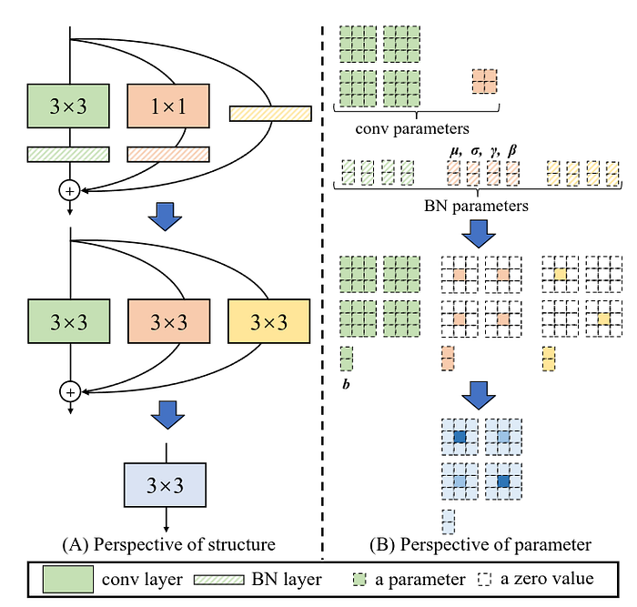
In the above, you can see that, after each Conv layer, we have a BatchNorm layer which are then fused to make single 3x3 Conv block. The authors have mentioned the foll. method to fuse them
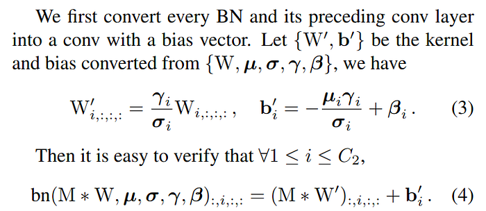
Fusing Conv2d and BatchNorm
def getBatchNormConvValues(conv, bn):
    batchNormMean, batchNormVariance, batchNormGamma, batchNormBeta = (bn.running_mean, bn.running_var, bn.weight, bn.bias)

    # Calulcate standard devitation
    batchNormStdDev = (batchNormVariance + bn.eps).sqrt()

    # Equation 3 from paper
    convBlock_weight = nn.Parameter((batchNormGamma/batchNormStdDev).reshape(-1, 1, 1, 1) * conv.weight)
    convBlock_bias = nn.Parameter(batchNormBeta - ((batchNormMean * batchNormGamma) / batchNormStdDev))

    return {"weight" : convBlock_weight, "bias" : convBlock_bias}

# Verify if we can Fuse Conv2d+BatchNorm to Conv2d
if __name__ == "__main__":

    convBlockWithBN = nn.Sequential(
        nn.Conv2d(16, 16, kernel_size=3, bias=False),
        nn.BatchNorm2d(16)
    )
    # convBlockWithBN[0] is nn.Conv2d and convBlockWithBN[1] is nn.BatchNorm

    # Random input
    # Batch size, Input channels, Height, Width
    input_x = torch.randn((1, 16, 32, 32))

    # Use uniform initialization technique to initialize the values of BatchNorm
    torch.nn.init.uniform_(convBlockWithBN[1].weight)
    torch.nn.init.uniform_(convBlockWithBN[1].bias)

    # Set block to eval mode
    convBlockWithBN.eval()

    with torch.no_grad():

        # Create a Conv2d block having in_channels, out_channels and kernel size from input
        fusedConvBNBlock = nn.Conv2d(convBlockWithBN[0].in_channels, convBlockWithBN[0].out_channels, convBlockWithBN[0].kernel_size)

        # get updated weight and bias values for Conv block
        getConvBNFusedValues = getBatchNormConvValues(convBlockWithBN[0],convBlockWithBN[1])

        # Load the updated weight and bias values to the fusedConvBNBlock block
        fusedConvBNBlock.load_state_dict(getConvBNFusedValues)

        # Check if PyTorch tensors are equal with marginal error of 0.000001 (1e-6)
        assert torch.allclose(convBlockWithBN(input_x), fusedConvBNBlock(input_x), atol=1e-6)
Now, we can use the above method to Fuse 3x3 Conv2d + BatchNorm to single 3x3 Conv2d. To convert 1x1 Conv2d + BatchNorm to single 3x3 Conv2d we can use the above Conv2d fusing method and then padding the tensor.
Converting Identity to 3x3 Conv2d
Identity layer just passes its input as output without any modification
# Code
input_x = torch.randn((1, 1, 3, 3))
identity = nn.Identity()

with torch.no_grad():
    identity.eval()
    print("Input : \n", input_x)
    print("Identity output : \n", identity(input_x))

# Output
Input :
tensor([[[[ 0.4986,  1.5723,  1.9968],
          [-0.4275,  1.2207, -0.3142],
          [ 1.7167, -0.1971,  0.5047]]]])
Identity output :
tensor([[[[ 0.4986,  1.5723,  1.9968],
          [-0.4275,  1.2207, -0.3142],
          [ 1.7167, -0.1971,  0.5047]]]])
Now, we need to replicate the same using Conv2d block.
In Identity block, all the values are Zero and the (in_channel, in_channel) is = 1.
For example, for a 2 channel, 4x4 Tensor, Identity block will look like follow :-
[
  [
     [
      [0., 0., 0.],
      [0., 1., 0.],
      [0., 0., 0.]],

     [
      [0., 0., 0.],
      [0., 0., 0.],
      [0., 0., 0.]
      ]
  ],

  [
    [
     [0., 0., 0.],
     [0., 0., 0.],
     [0., 0., 0.]
    ],
    [
      [0., 0., 0.],
      [0., 1., 0.],
      [0., 0., 0.]
    ]
  ]
]
Now, lets create a Conv2d block whose weights are same like above
# Create a Conv2d block with padding 1 to maintain the input size
conv = nn.Conv2d(in_channels=2, out_channels=2, kernel_size=3, padding=1, bias=False)

# Make weights of the Conv block as 0
conv.weight.zero_()

# Iterate over Conv channels, and only set (in_channel, in_channel) = 1
for i in range(conv.in_channels):
  conv.weight[i, i % conv.in_channels, 1, 1] = 1
Now, if I pass a 3x3 input, the output will be same as input
# For input
input_x = torch.randn((1, 2, 4, 4))

# Output is
Input Tensor :
 tensor([[[[-0.0538,  0.5682, -0.6977, -0.9699],
          [ 0.3265,  0.5746,  0.5554, -0.7832],
          [-0.4921, -0.5943,  1.7714, -0.9190],
          [-0.4241, -0.3623, -0.0454, -0.2908]],

         [[ 0.8274,  0.0891, -1.3426, -1.9100],
          [ 1.2594, -0.6410, -0.8667,  2.2247],
          [-0.7273,  0.3608, -0.2968,  0.5505],
          [ 1.6419,  0.2357,  1.6606, -0.2523]]]])
Conv Identity output :
 tensor([[[[-0.0538,  0.5682, -0.6977, -0.9699],
          [ 0.3265,  0.5746,  0.5554, -0.7832],
          [-0.4921, -0.5943,  1.7714, -0.9190],
          [-0.4241, -0.3623, -0.0454, -0.2908]],

         [[ 0.8274,  0.0891, -1.3426, -1.9100],
          [ 1.2594, -0.6410, -0.8667,  2.2247],
          [-0.7273,  0.3608, -0.2968,  0.5505],
          [ 1.6419,  0.2357,  1.6606, -0.2523]]]])
Variants of RepVGG
RepVGG has 5 blocks of 3x3 layers. To perform Image Classification, Global Average Pooling is used before passing features to Fully connected layers.
Quoting from the paper as its explained clearly
“We decide the numbers of layers of each stage following three simple guidelines. 1) The first stage operates with large resolution, which is time-consuming, so we use only one layer for lower latency. 2) The last stage shall have more channels, so we use only one layer to save the parameters. 3) We put the most layers into the second last stage (with 14 × 14 output resolution on ImageNet), following ResNet and its recent variants. We let the five stages have 1, 2, 4, 14, 1 layers respectively to construct an instance named RepVGG-A. We also build a deeper RepVGG-B, which has 2 more layers in stage2, 3 and 4. We use RepVGG-A to compete against other lightweight and middleweight models including ResNet-18/34/50, and RepVGG-B against the high-performance ones”
Results

The above table shows how well RepVGG is performing compared to other available SOTA. Please go through the Experiments section to know more about its performance.
Thanks for reading. For more such blogs, do follow me on Medium and also connect with me on LinkedIn :)